Excel Macro: Evaluating Formulas Dynamically

In this post, we will see how excel formulas can be picked-up dynamically in excel macros. This tutorial also covers applying cell formats dynamically.

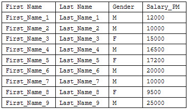
Lets consider the following example. For data setup, we open a new excel file and create a worksheet named “Data” in it. We set up the following sample data set in this sheet.

The requirement is to write a macro which will populate additional columns based on some calculations (apply formulas on the existing data cells) for all the rows present. So, the result would look something like:

The following processing has been done:

' Two new columns “Full Name” and “Bonus” have been added.
 
' The value for “Full name” has been computed based on following formula:
  IF(C2 = "M", "Mr ","Mrs ") & A2 & " " &B2
 
' The value for “Bonus” has been calculated based on the following formula:
  (D2 * 12) * (10/100)
  where the bonus is 10% of the annual salary.

' A specific formatting has been applied to the bonus value.
 
' The values have been computed for the whole range of data ( 9 rows in this case).
Code language: PHP (php)

The task is to achieve this whole processing via an excel macro. Further, we will try to keep all the aspects as dynamic as possible. For this, we create another worksheet named “Config” and populate the following data in it:

So, each formula being used in the calculation is mentioned as a configuration in this new sheet. Also, the bonus value has been mentioned as 10% (It can also be made a configuration item where we read it from another cell). Please note that the formula contains 2nd row references. We will shortly see the reason for that.

Save this workbook as “dynamic_macro.xlsm”. The extension “.xlsm” is used for macro enabled workbooks.

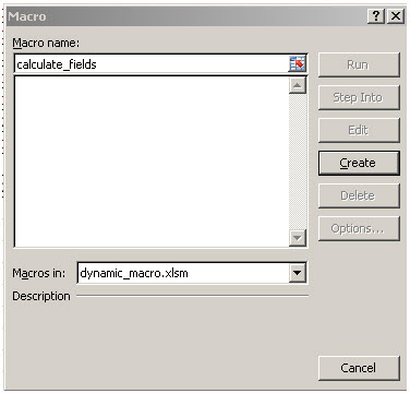
Now that we are done defining the problem statement and doing the required data setup, let’s move on to writing the macro. Under the “Developer” tab in Menu, click on “Macros”. The following dialogue box will open, just put a macro name and click on “create”.

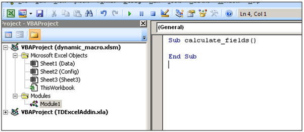
Once you click on “create” button, it will open a VB editor where the coding can be done:

Simply copy-paste the below code in the above editor:

' Function to return string based on the integer value passed for columns (For Ex: AA, A, HR etc.)
Function ColLtr(iCol As Integer) As String
    If iCol > 0 And iCol <= Columns.Count Then
        ColLtr = Evaluate("substitute(address(1, " & iCol & ", 4), ""1"", """")")
    End If
End Function

' Main procedure for the processing
Sub calculate_fields()
   ' Defining the worksheet names
    strData = "Data"
    srtConfig = "Config"

    ' Getting the worksheet handle
    Set wsData = ThisWorkbook.Worksheets(strData)
    Set wsConfig = ThisWorkbook.Worksheets(srtConfig)

    ' Activating the "Data" worksheet
    wsData.Activate

    ' Getting the row / column count of existing data.
    dataRowCount = wsData.UsedRange.Rows.Count
    dataColCount = wsData.UsedRange.Columns.Count

    ' Getting the formula row count in "Config" worksheet, substracting 1 for the header records
    formulaRowCount = wsConfig.Range("A1").End(xlDown).Row - 1

    ' Looping through the config rows count. In this setup, these are the columns to be computed
    For i = 1 To formulaRowCount
        ' Copy the column header name from column "B"
        Cells(1, dataColCount + i) = wsConfig.Range("B" & (i + 1)).Value

        ' Get the column format (if any)
        colFormat = wsConfig.Range("D" & (i + 1)).Value

        ' Applying the formula to the 2nd row after the actual column count in the "Data" worksheet
        Range(ColLtr(dataColCount + i) & "2").Formula = "=" & Replace(wsConfig.Range("C" & (i + 1)).Value, "", """")

        ' Apply the formatting (if specified)
        If colFormat  "" Then
            ' Replace any " in the format value with ""
            colFormat = Replace(colFormat, """", """""")
            Range(ColLtr(dataColCount + i) & "2").NumberFormat = colFormat
        End If

        ' Noting the range start value
        If i = 1 Then
            strCopyStart = ColLtr(dataColCount + i)
        End If

        ' Noting the range end value
        If i = formulaRowCount Then
            strCopyEnd = ColLtr(dataColCount + i)
        End If
    Next i

    ' Selecting the range for which the formulas have been applied
    Range(strCopyStart & "2:" & strCopyEnd & "2").Select

    ' Using Autofill to apply formula to all the records
    copyRange = strCopyStart & "2:" & strCopyEnd & (dataRowCount)
    Selection.AutoFill Destination:=Range(copyRange), Type:=xlFillDefault

    ' Finally, save the workbook
    ThisWorkbook.Save

End Sub
Code language: HTML, XML (xml)

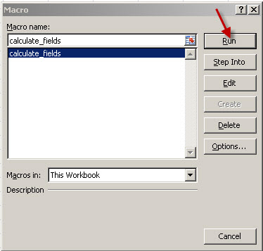
Once done, save the code changes. It will take you back to the following screen where you can just select and run the macro.

Let’s now go through the code and try to understand the functionality.

The generic function “ColLtr” is useful to get the cell in lettered format. For Ex:

5 will return E
27 will return AA
55 will return BC and so on
Code language: JavaScript (javascript)

In the main procedure, we defined the worksheets name, got their handles and activated the “Data” worksheet. The “UsedRange” property has been used to get the rows and columns count.

dataRowCount = wsData.UsedRange.Rows.Count
dataColCount = wsData.UsedRange.Columns.Count

Every Worksheet object has a UsedRange property that returns a Range object representing the area of a worksheet that is being used. The UsedRange property represents the area described by the farthest upper-left and farthest lower-right nonempty cells in a worksheet and includes all cells in between. Because the test data in our case is continuous, it can be used directly to get the count.

You might use the UsedRange property together with the SpecialCells method to return a Range object representing all cells in a worksheet of a specified type. For example, the following code returns a Range object that includes all the cells in the active worksheet that contain a formula:

Dim rngFormulas As Excel.Range
Set rngFormulas = ActiveSheet.UsedRange.SpecialCells(xlCellTypeFormulas)
Code language: JavaScript (javascript)

On the next line, a different property “Range.End” has been used to get the row count.

formulaRowCount = wsConfig.Range("A1").End(xlDown).Row - 1
Code language: HTML, XML (xml)

This property returns a Range object that represents the cell at the end of the region that contains the source range. The generic syntax for this property is:

expression.End(Direction)
Code language: CSS (css)

Where, expression is a variable that represents a Range object. The parameter “Direction” mentions the direction in which to move. The valid values are:

xlDown ' Down
xlToLeft ' To Left
xlToRight ' To Right
xlUp ' Up
Code language: PHP (php)

Once the formula count is there, we just loop that many times to get the additional columns created. Within the loop, the column header has been copied as mentioned in the “Config” worksheet by using the “Range.Value” property:

Cells(1, dataColCount + i) = wsConfig.Range("B" & (i + 1)).Value
Code language: JavaScript (javascript)

Similarly, the format which has to be applied to this new column is fetched.

Now, this is the most interesting part of the code where we apply the formula to column:

' Applying the formula to the 2nd row after the actual column count in the "Data" worksheet
Range(ColLtr(dataColCount + i) & "2").Formula = "=" & Replace(wsConfig.Range("C" & (i + 1)).Value, "", """")

Here, the “Range.Formula” property is used. If the cell contains a constant, this property returns the constant. If the cell is empty, this property returns an empty string. If the cell contains a formula, the Formula property returns the formula as a string in the same format that would be displayed in the formula bar (including the equal sign (=)).

So, to set formula for this cell, we prefix the formula value which is picked from the “Config” by “=”. Also note that double quotes in the actual formula has to be escaped to preserve it. In case any change in formula is required, we just need to update the details on “Config” worksheet and the changes will reflect automatically with the next run.

The format, if any, is then applied to the cell. Again, because we are reading this format from “Config”, the double quotes have to be escaped.

' Apply the formatting (if specified)
        If colFormat  "" Then
            ' Replace any " in the format value with ""
            colFormat = Replace(colFormat, """", """""")
            Range(ColLtr(dataColCount + i) & "2").NumberFormat = colFormat
        End If
Code language: PHP (php)

The “Range.NumberFormat” property has been used for doing that. This property returns or sets a Variant value that represents the format code for the object. The format code is the same string as the Format Codes option in the Format Cells dialog box. Here are few more examples:

Worksheets("Sheet1").Range("B13").NumberFormat = "General"               ' 35332
Worksheets("Sheet1").Rows(5).NumberFormat = "[$-409]m/d/yy h:mm AM/PM;@" ' 5/2/2014  12:00:00 AM
Worksheets("Sheet1").Columns("C"). _ 
 NumberFormat = "$#,##0.00_);[Red]($#,##0.00)"                           ' USD 45,123,234.00
Code language: PHP (php)

Finally, the whole range of the new columns have been selected (2nd row as the 1st one is just header) and applied to all the rows.

' Using Autofill to apply formula to all the records
    copyRange = strCopyStart & "2:" & strCopyEnd & (dataRowCount)
    Selection.AutoFill Destination:=Range(copyRange), Type:=xlFillDefault

I hope you have found this post useful. Although there are several other ways in VB to accomplish the same tasks, what I have tried here is to provide a working solution for a particular use case which can be generalised based on requirements. As some of you must have already noticed, I haven’t bothered to make this macro re-runnable. But that can be easily achieved; in my use case, I was refreshing the whole data from other workbook before running the macro.

References:
https://msdn.microsoft.com/en-us/library/office